Quantitative Risk Analysis: Methods, Formula & Examples

Quantitative risk analysis is a method that measures risk in numerical, often monetary, terms by combining the probability of an event with the size of its impact. Instead of labeling a risk "high" or "low," it produces figures such as a $250,000 expected annual loss or a 15 percent chance of a six-month delay. Security, project, and finance teams use those numbers to compare risks on a common scale, justify budgets, and decide which exposures to treat first.

The approach applies across cybersecurity, project management, finance, insurance, and engineering. NIST Special Publication 800-30 treats quantitative analysis as one of three assessment approaches, alongside qualitative and semi-quantitative, and the choice depends on the data available and the decision at stake.

This guide covers how quantitative risk analysis works, how it differs from qualitative analysis, the main methods and their formulas, a worked cyber example, and where the approach helps and where it falls short.

What is Quantitative Risk Analysis?

Quantitative risk analysis assigns measurable values to two variables for every risk: the probability that an event occurs, and the impact, expressed in money, time, or another unit, if it does. Multiplying or modeling those two variables produces a risk exposure figure that ranks risks objectively against one another.

As the ISACA Journal frames it, quantitative analysis assigns objective numerical or measurable values rather than descriptive ratings. The outputs take several forms depending on the field: an annualized loss expectancy in cybersecurity, a contingency reserve in project management, or a value at risk in finance. Each translates uncertainty into a number that decision-makers and boards act on.

Qualitative vs. Quantitative Risk Analysis

Qualitative and quantitative analyses answer different questions. Qualitative analysis sorts risks quickly using descriptive scales, while quantitative analysis measures them precisely using data and models. The table contrasts the two approaches across the dimensions that matter most.

Dimension	Qualitative Risk Analysis	Quantitative Risk Analysis
Output	Descriptive ratings (high, medium, low)	Numeric values (dollars, percentages, time)
Inputs	Expert judgment and ranking	Data, probability distributions, models
Objectivity	Subjective, prone to bias	Objective, repeatable
Speed and Cost	Fast and inexpensive	Slower and resource-intensive
Data Needed	Little historical data	Reliable historical or estimated data
Best For	Screening and prioritizing many risks	High-stakes decisions needing financial precision

The two approaches complement each other rather than compete. Mature programs run a fast qualitative pass to surface and rank risks, then apply quantitative analysis to the few that carry enough financial weight to justify the effort. Blending the two, sometimes called a semi-quantitative approach, gives both breadth and precision.

How to Perform Quantitative Risk Analysis

A quantitative analysis follows a repeatable sequence. Each step converts judgment and raw data into a defensible number.

1. Identify and Catalog Risks

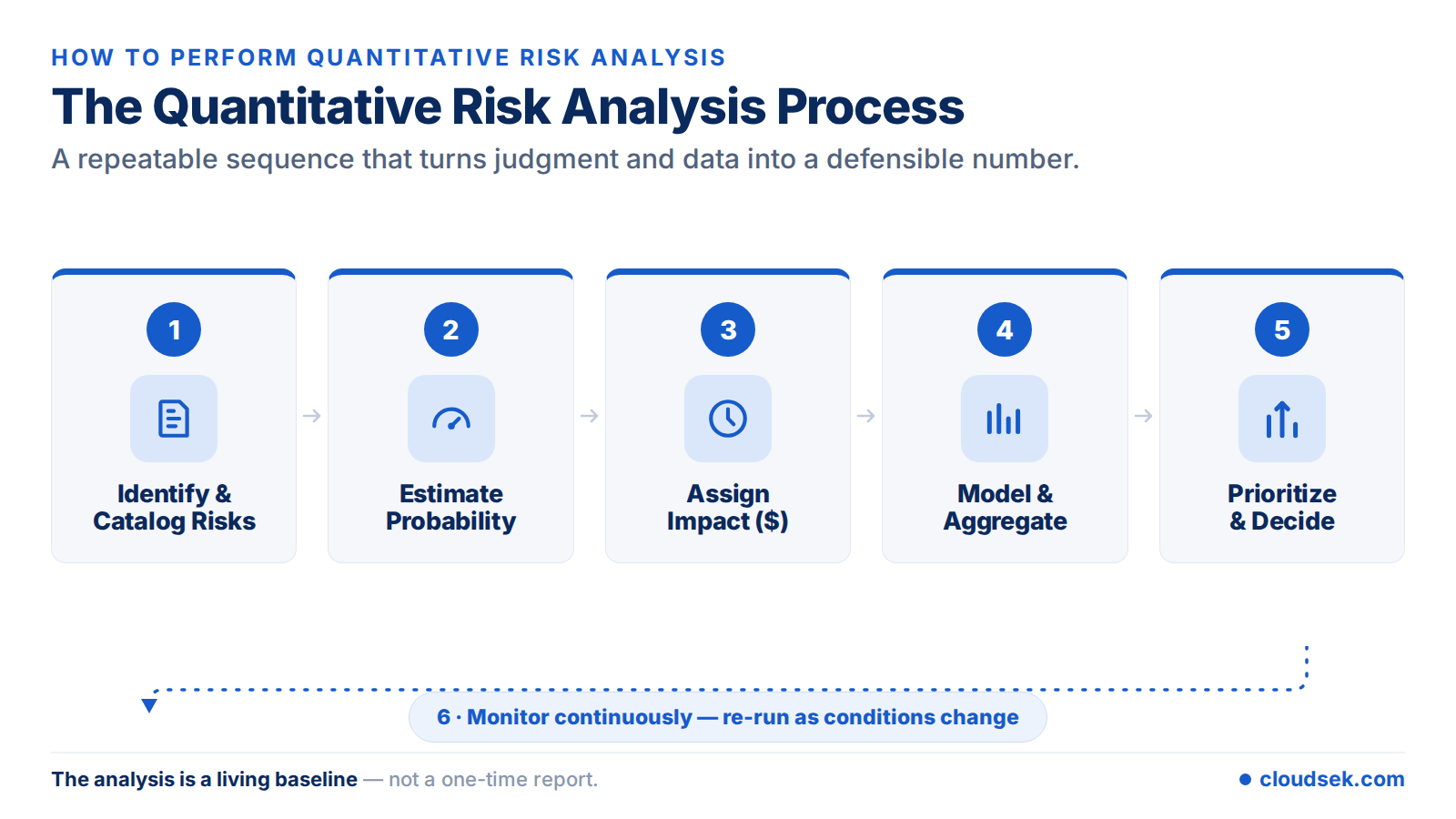
List the risks that could affect the asset, project, or organization, and record them in a risk register. A quantitative analysis typically inherits this list from an earlier qualitative screening that has already filtered out low-priority items. Common categories include data breaches, schedule delays, supplier failures, and equipment faults.

2. Estimate Probability

Assign each risk a likelihood, drawn from historical data, industry benchmarks, or structured expert estimates. Probability can be a single percentage or a full distribution that captures the range of plausible frequencies. The quality of this input determines the credibility of every figure that follows.

3. Assign Impact in Measurable Terms

Quantify the consequence of each risk in money, time, or another concrete unit. In cybersecurity, this means estimating breach costs such as response, downtime, fines, and lost customers. Recording impact as a value rather than a label is what separates quantitative analysis from a qualitative matrix.

Impact often spans direct costs that are straightforward to count and indirect costs, such as reputational damage, that demand judgment to estimate.

4. Model and Aggregate

Combine probability and impact using a method suited to the data, such as expected monetary value for discrete risks or Monte Carlo simulation for interacting ones. Aggregation shows how individual risks roll up into total exposure, since several moderate risks can together outweigh a single severe one. Correlated risks need extra care, because events that tend to occur together raise the odds of a severe combined outcome.

5. Prioritize and Decide

Rank risks by their quantified exposure and use the figures to set contingency reserves, compare mitigation options, and make go or no-go calls.

A risk with a high expected loss and an affordable control becomes an obvious early target, while a low-exposure risk can be accepted and documented. Quantified numbers give boards and regulators a clear, comparable basis for security and investment decisions.

6. Monitor Continuously

Treat the analysis as a living baseline rather than a one-time report. As new loss data, threats, and exposures emerge, the numbers shift, so periodic re-runs keep priorities aligned with current conditions and measure whether controls are working.

Quantitative Risk Analysis Methods and Techniques

Several techniques turn probability and impact into numbers. The right one depends on whether risks are discrete or continuous, how much data exists, and the precision the decision requires.

Method	How it works
Annualized Loss Expectancy (ALE)	ALE = SLE × ARO, where single loss expectancy (SLE) = asset value × exposure factor, and ARO is the annual rate of occurrence. The standard cybersecurity loss formula.
Monte Carlo Simulation	Runs thousands of randomized iterations across input distributions to produce a full range of possible outcomes and their probabilities.
Expected Monetary Value (EMV)	EMV = sum of (probability × impact) across outcomes, used to forecast the cost of a decision or project with risk factored in.
Decision Tree Analysis	Maps choices and chance events as branches, multiplies each branch probability by its value, and compares paths to find the lowest-risk option.
Three-Point Estimate / PERT	Combines optimistic (O), most likely (M), and pessimistic (P) estimates. PERT weights the middle: expected value = (O + 4M + P) / 6.
Sensitivity Analysis	Varies one input at a time to rank which variables move the outcome the most, often shown as a tornado diagram.
FAIR	Factor Analysis of Information Risk: risk = loss event frequency × loss magnitude, producing a financial estimate of cyber risk.
Failure Mode and Effects Analysis (FMEA)	Scores each failure mode by severity, occurrence, and detection; the product is a risk priority number (RPN).

Monte Carlo simulation often sits underneath the others, since it can run an ALE or FAIR model thousands of times to convert single-point estimates into a probability distribution. That distribution reveals not just an average loss but the odds of a worst-case outcome.

Worked Example: Expected Monetary Value

Expected monetary value shows how these methods produce a usable number. Suppose a project faces two risks: a supplier delay with a 30 percent probability and a $200,000 impact, and an equipment fault with a 10 percent probability and a $500,000 impact.

The expected monetary value of the delay is 0.30 x $200,000, or $60,000, and the fault is 0.10 x $500,000, or $50,000. Summed, the project carries $110,000 of risk-adjusted cost, which the team sets aside as a contingency reserve. The same arithmetic ranks the delay above the fault despite its smaller worst-case loss.

Quantitative Risk Analysis in Cybersecurity

In cybersecurity, quantitative risk analysis is known as cyber risk quantification, and it translates technical exposures into financial terms a board understands. Two models dominate: the annualized loss expectancy formula for quick estimates, and the FAIR model for detailed, defensible analysis. CloudSEK's guide to cyber risk quantification frameworks notes that regulators, including the SEC since 2023, now expect this kind of financial framing of cyber risk.

The ALE Formula, With a Worked Example

Annualized loss expectancy expresses the average yearly cost of a risk. It builds on two inputs: single loss expectancy (SLE), the cost of one incident, and the annual rate of occurrence (ARO), how often the incident happens per year.

SLE = Asset Value x Exposure Factor | ALE = SLE x ARO

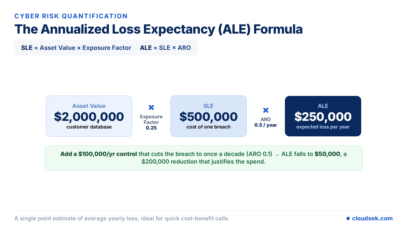
Consider a customer database valued at $2,000,000. A breach is estimated to compromise 25 percent of that value, so the exposure factor is 0.25 and the single loss expectancy is $500,000. If such a breach is expected once every two years, the annual rate of occurrence is 0.5, giving an annualized loss expectancy of $250,000.

A proposed control costing $100,000 a year that cuts the occurrence rate to once a decade lowers the ALE to $50,000, a $200,000 reduction that justifies the spend. This is how quantitative analysis turns a security decision into a cost-benefit calculation.

The FAIR Model

The FAIR model (Factor Analysis of Information Risk), maintained as a standard by the Open Group, breaks risk into loss event frequency and loss magnitude. Loss event frequency combines threat event frequency with vulnerability, while loss magnitude adds primary losses, such as response and downtime, to secondary losses, such as fines and reputational damage.

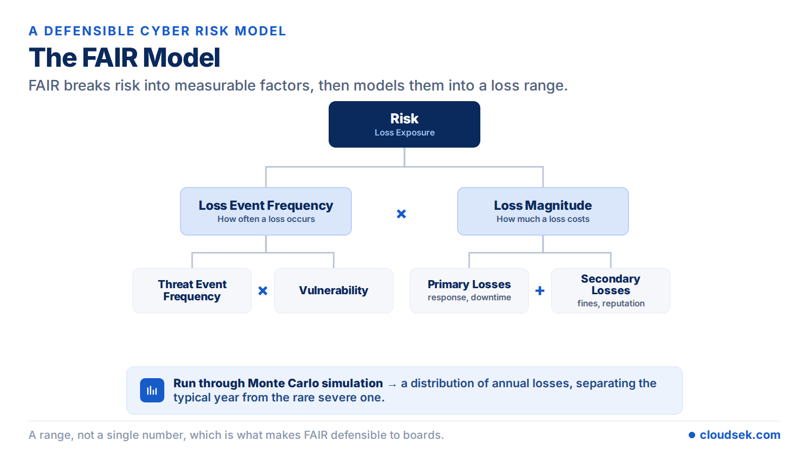
Analysts feed these factors through a Monte Carlo simulation to produce a financial range rather than a single number. The same likelihood and exposure data behind a data risk assessment feeds directly into these models, which is why accurate visibility of assets and threats improves the quality of the result.

A FAIR result is therefore a distribution, separating the typical annual loss from the rare but severe one that a single average would hide.

Benefits of Quantitative Risk Analysis

Expressing risk in numbers changes how an organization makes decisions. The main advantages are concrete:

Objective decisions: figures based on data reduce the bias and inconsistency of subjective ratings.
Sharper prioritization: a common numeric scale ranks risks directly, so resources flow to the largest exposures first.
Financial planning: quantified losses, set contingency reserves, and support cost-benefit analysis of controls.
Board communication: dollar figures give technical and non-technical stakeholders a shared language for risk.
Measurable monitoring: numbers create a baseline that tracks whether risk and control effectiveness improve over time.

Limitations and Challenges of Quantitative Risk Analysis

The precision of quantitative analysis carries trade-offs that shape when it makes sense to use.

Data dependency: credible figures need reliable historical or loss data, which many organizations lack for rare events.
Complexity and expertise: models such as Monte Carlo and FAIR require statistical skill and time to build and defend.
False precision: a number looks authoritative even when its inputs are rough guesses, so weak estimates can mislead.
Cost and effort: the analysis consumes resources that a fast qualitative review would not, making it overkill for minor risks.
Point-in-time validity: estimates reflect the data available when the analysis runs, so figures age as threats, asset values, and conditions change.

For these reasons, quantitative analysis complements qualitative analysis rather than replacing it. Teams reserve the heavier method for the decisions where a precise number changes the outcome.

Quantitative Risk Analysis Tools and Frameworks

Established frameworks supply the structure, and software supplies the computation. NIST SP 800-30 defines the qualitative, semi-quantitative, and quantitative approaches for information security. The FAIR standard and the Open Group Risk Taxonomy provide the model for cyber risk quantification.

The CIS Risk Assessment Method (CIS RAM) and the PMBOK Perform Quantitative Risk Analysis process apply the discipline to security controls and projects. Monte Carlo simulation tools, including spreadsheet add-ins, run the underlying probability models, and dedicated cyber risk quantification platforms automate FAIR-based analysis at scale.

Frequently Asked Questions

What is the formula for quantitative risk analysis?

The most common formula is annualized loss expectancy: ALE = SLE x ARO, where single loss expectancy equals asset value times exposure factor. For project risks, expected monetary value sums probability times impact across outcomes.

Is Monte Carlo simulation qualitative or quantitative?

Quantitative. Monte Carlo simulation runs thousands of numerical iterations across probability distributions to produce a measurable range of outcomes, making it one of the core quantitative risk analysis techniques.

When should you use quantitative risk analysis?

Use it for high-stakes decisions where a precise financial figure changes the outcome, such as justifying a security budget or a major investment, and where reliable data exists to support the estimates.

What is quantitative risk analysis in project management?

It is the PMBOK process that assigns numerical values to identified project risks to forecast cost and schedule impact, using techniques such as Monte Carlo simulation, decision trees, and three-point estimates to set contingency reserves.

What data do you need for quantitative risk analysis?

Two inputs per risk: the probability or frequency of the event, and its impact in money or time. Both draw on historical loss data, industry benchmarks, asset values, and structured expert estimates.

Which is better, qualitative or quantitative risk analysis?

Neither is better; they serve different purposes. Qualitative analysis screens and ranks many risks quickly, while quantitative analysis measures the critical few precisely. Most programs use qualitative first, then quantitative, on the risks that warrant it.